import matplotlib.pyplot as plt
from sklearn.model_selection import learning_curve
pipe_lr = make_pipeline(StandardScaler(),
LogisticRegression(penalty='l2',
random_state=1,
solver='lbfgs',
max_iter=10000))
train_sizes, train_scores, test_scores = learning_curve(estimator=pipe_lr,
X=X_train,
y=y_train,
train_sizes=np.linspace(0.1, 1.0, 10),
cv=10,
n_jobs=1)
train_mean = np.mean(train_scores, axis=1)
train_std = np.std(train_scores, axis=1)
test_mean = np.mean(test_scores, axis=1)
test_std = np.std(test_scores, axis=1)
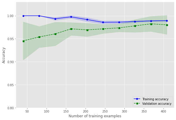
plt.style.use('ggplot')
plt.plot(train_sizes, train_mean,
color='blue', marker='o',
markersize=5, label='Training accuracy')
plt.fill_between(train_sizes,
train_mean + train_std,
train_mean - train_std,
alpha=0.15, color='blue')
plt.plot(train_sizes, test_mean,
color='green', linestyle='--',
marker='s', markersize=5,
label='Validation accuracy')
plt.fill_between(train_sizes,
test_mean + test_std,
test_mean - test_std,
alpha=0.15, color='green')
# plt.grid()
plt.xlabel('Number of training examples')
plt.ylabel('Accuracy')
plt.legend(loc='lower right')
plt.ylim([0.8, 1.03])
plt.show()